Designing a database schema is a foundational skill for any engineer working with structured data. While Entity-Relationship Diagrams (ERDs) are taught extensively in university courses, the transition from a theoretical model to a live, high-traffic production environment introduces complex challenges. This guide explores the practical application of ERD principles, highlighting where academic perfection meets engineering reality. We will examine how to maintain data integrity while optimizing for performance, scalability, and maintainability without relying on specific vendor tools.
Understanding the gap between a clean diagram and a deployed system requires a shift in mindset. In academia, the focus is often on normalization and theoretical correctness. In production, factors like query latency, write throughput, and disaster recovery become equally critical. This article provides a deep dive into bridging that divide, ensuring your data models are robust enough to handle real-world demands.
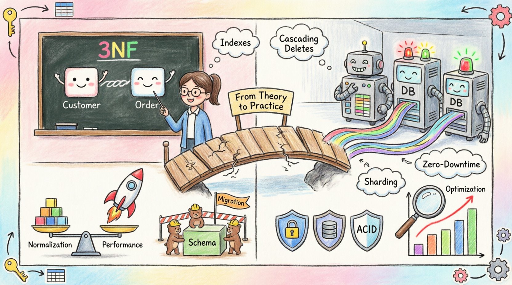
🎓 The Academic Foundation Revisited
Before addressing production nuances, we must establish what the standard academic approach entails. An Entity-Relationship Diagram typically defines entities, attributes, and relationships. These components form the blueprint for relational databases.
Core Components
- Entities: Represent real-world objects or concepts, such as a Customer or an Order.
- Attributes: Properties describing the entities, like Name, ID, or CreatedDate.
- Relationships: Connections between entities, defined by cardinality (One-to-One, One-to-Many, Many-to-Many).
In a classroom setting, the goal is often to achieve Third Normal Form (3NF). This eliminates redundancy and ensures data consistency. Every non-key attribute depends on the key, the whole key, and nothing but the key. While this is logically sound, it does not account for the physical cost of accessing data.
🚀 The Production Environment Shift
When moving to a live system, the constraints change dramatically. You are no longer designing for a single user on a local machine. You are designing for millions of users, network partitions, and hardware failures. The academic model often assumes ideal conditions that rarely exist in the wild.
Key Differences
| Aspect | Academic Model | Production Reality |
|---|---|---|
| Performance | Query optimization is secondary | Latency is a primary constraint |
| Integrity | Strict referential integrity enforced | May be relaxed for availability |
| Scale | Single node assumed | Horizontal scaling required |
| Changes | Static schema | Continuous evolution and migration |
For instance, a strict 3NF design might require joining five tables to retrieve a simple report. In a production environment with high read traffic, these joins can become a bottleneck. The database engine must lock multiple rows, increasing contention. Engineers often accept a degree of redundancy to avoid these expensive operations.
🔗 Modeling Relationships Under Load
Relationships are the backbone of relational data. However, implementing them in a production system requires careful consideration of foreign keys and constraints. The academic model treats relationships as static links, but in practice, they are dynamic pathways for data access.
One-to-Many Relationships
This is the most common pattern. A single Parent record relates to multiple Child records. In production, this introduces specific challenges:
- Indexing: The foreign key column on the Child table must be indexed. Without this, queries filtering by the Parent become full table scans.
- Deletion Cascades: If a Parent is deleted, what happens to the Children? Automatic cascading deletes can lead to accidental data loss if not carefully managed. Sometimes, soft deletes are preferred to preserve history.
- Write Amplification: Every insert into a Child table requires a write to the Parent index to maintain the relationship. High write volumes can impact the index performance.
Many-to-Many Relationships
Academic diagrams show a direct link between two entities. In a database, this requires a junction table. In production, this junction table becomes a critical choke point.
- Cardinality Limits: If a junction table grows to billions of rows, querying becomes slow. Partitioning strategies must be applied.
- Transaction Scope: Updating relationships often involves multiple tables. Ensuring atomicity across these tables requires careful transaction management.
- Query Complexity: Retrieving data from many-to-many relationships often requires multiple joins. In high-traffic systems, denormalizing this data into a single table might be more efficient.
⚖️ Normalization vs. Performance Trade-offs
Normalization reduces data duplication, but it increases the complexity of retrieval. Denormalization does the opposite. The decision to normalize or denormalize is one of the most critical architectural choices in database design.
When to Denormalize
There are specific scenarios where breaking the rules of normalization is justified:
- Read-Heavy Workloads: If your application reads data far more often than it writes, storing pre-joined data can save CPU cycles and I/O operations.
- Reporting and Analytics: Data warehouses often use star schemas, which are highly denormalized, to speed up aggregation queries.
- Sharding Constraints: When data is split across multiple servers, joining tables across shards is expensive or impossible. Keeping related data on the same shard requires duplication.
Risks of Denormalization
While performance improves, data integrity becomes harder to maintain.
- Update Anomalies: If you change a value in one place, you must update it in all denormalized copies. Missing one copy leads to inconsistent data.
- Storage Costs: Redundant data consumes more disk space. While cheap, it adds up at scale.
- Write Latency: Writing more data per transaction increases the time required to commit changes.
🛠 Schema Evolution and Migration
In academia, a schema is designed, implemented, and finalized. In production, a schema is a living organism that changes constantly. Features are added, requirements shift, and bugs are fixed. This necessitates a robust migration strategy.
Zero-Downtime Migrations
Changing a schema usually requires locking the table, which stops service. In a 24/7 environment, this is unacceptable. Strategies include:
- Expand and Contract: Add the new column first. Populate it in the background. Then, switch the application to read the new column. Finally, remove the old column.
- Backfilling: When adding data to a new column, ensure existing rows are updated. This can be done in small batches to avoid locking the table for long periods.
- Virtual Columns: Some systems allow computed columns that derive values from existing data, allowing for a smooth transition without physical changes.
Handling Divergent Versions
During a migration, the system might run multiple versions of the schema simultaneously. The application code must be backward compatible. This means:
- Old code must work with the new schema.
- New code must work with the old schema.
- Both versions must coexist until the migration is complete.
🔒 Data Integrity Constraints
Database constraints are designed to protect data quality. However, enforcing them strictly can impact performance. Understanding where to apply constraints is key.
Types of Constraints
- Primary Keys: Uniquely identify a row. Always enforce this. It is fundamental to the structure.
- Foreign Keys: Ensure relationships exist. These can be expensive to check on every insert or update. Consider deferring checks if performance is critical.
- Check Constraints: Validate specific values, such as age > 0. These are usually cheap to enforce.
- Unique Constraints: Ensure no duplicates. Useful for emails or usernames. Requires indexing.
Application vs. Database Layer
Where should validation logic live? Placing it in the application layer is faster but less safe. Placing it in the database layer is safer but slower. The best approach is often a hybrid:
- Use database constraints for critical integrity rules (like Primary Keys and Foreign Keys).
- Use application logic for complex business rules (like “User cannot place an order if they have an unpaid invoice”).
📊 Monitoring and Maintenance
Once the system is live, the work is not done. You must monitor the health of the data model. An ERD is a snapshot in time; a production database is a dynamic state.
Key Metrics to Track
- Index Usage: Unused indexes waste resources. Identify and remove them periodically.
- Fragmentation: Over time, data pages become fragmented. Rebuilding indexes can restore performance.
- Lock Contention: Monitor for queries that hold locks for too long, blocking other operations.
- Table Growth: Predict how fast tables will grow to plan capacity.
Audit Trails
For compliance and debugging, you need to know who changed what and when. Implementing an audit table or using system features to log changes is essential. This helps trace back data issues to their source.
🏁 Moving Forward
Bridging the gap between academic ERD concepts and production systems requires a pragmatic approach. It involves understanding that data modeling is not just about correctness; it is about efficiency, resilience, and adaptability. By balancing normalization with performance needs, planning for schema evolution, and enforcing integrity wisely, you can build systems that stand the test of time.
Remember that every design decision has a trade-off. There is no perfect schema, only the right schema for the specific context. Continuously review your data models against real-world usage patterns. Adjust indexes, refine relationships, and evolve your architecture as your data grows. This iterative process ensures your system remains robust and responsive.